Chapter 27 Visual Comparisons of Data with a Normal Model
Welcome back to Quantitative Reasoning! In our previous tutorial, we learned how to compute numeric predictions from a normal model. Many real-world data can be approximated by a normal model, but there are also many cases where a normal model is a poor fit. In this tutorial, we learn two visualisation techniques that can help us decide whether a normal model is appropriate for our data:
- The first technique is to plot the probability density of a normal model (i.e. the “bell curve”) on top of a histogram of the data.
- The second technique is to make a so-called “normal probability plot”, also known as Q-Q plot.
As a test case, we can use data that are guaranteed to come from a normal
model: random numbers generated with rnorm().
Let’s make a histogram of 10,000 random numbers.
r <- rnorm(10000, mean = 500, sd = 100)
hist(r)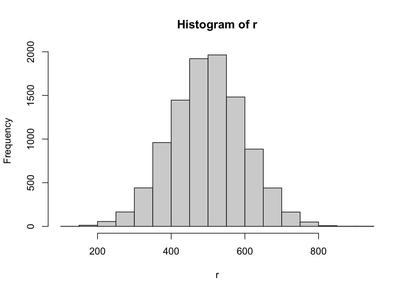
If we want to compare the histogram with a bell curve plotted with dnorm(),
we must normalize the histogram so that the combined area of all bins is equal
to 1.
That is, the height of each bin should not be the number of data points
(also called “frequency”) in that bin.
Instead we must scale the bin heights by an appropriate factor so that the
total area in the bins equals 1.
A convenient way to accomplish this task is to pass the argument
freq = FALSE to the hist() function.
Note the different y-axis tick marks in the previous and the following
plot.
hist(r, freq = FALSE)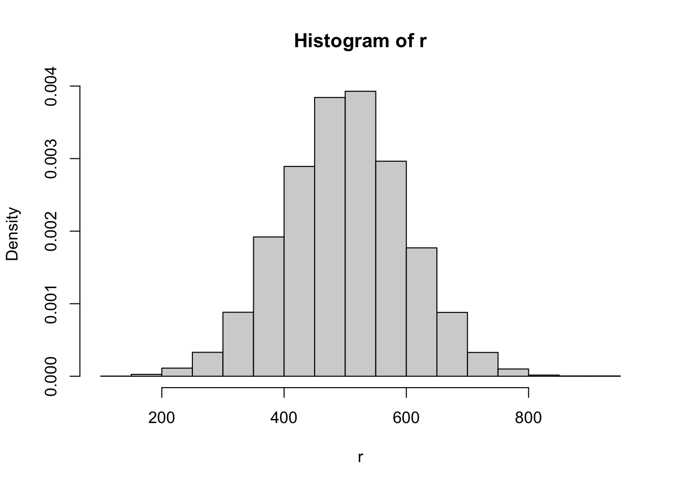
We can add the bell curve to the plot with the curve() function.
To put the curve on top of the existing plot, we must use the argument
add = TRUE.
hist(r, freq = FALSE)
curve(dnorm(x, mean = 500, sd = 100),
      from = 200,
      to = 800,
      add = TRUE,
      col = "red")
For our random numbers, the heights of the histogram bins are almost exactly on
the bell curve.
This result isn’t surprising because we used rnorm(), so the numbers came
from the normal model whose probability density is shown by the red curve.
The situation is often less clear-cut when working with real data. Let’s consider a data set that our textbook uses as an example. Below this video, you find a link to a spreadsheet with results from the 2001-2002 US National Health and Nutrition Examination Survey (NHANES, https://michaelgastner.com/data_for_QR/nhanes_dvvb_ch5.csv). The spreadsheet has two columns. The first column shows a numeric ID for all 19-24 year-old men with a height between 172 cm and 178 cm who participated in the survey. The second column shows their weight in kilograms.
nhanes_dvvb_ch5 <- read.csv("nhanes_dvvb_ch5.csv")
head(nhanes_dvvb_ch5)
## id weight
## 1 10153 95.7
## 2 10461 68.9
## 3 10516 60.3
## 4 10566 60.4
## 5 10765 69.7
## 6 11253 59.1Let’s draw a histogram of the weight with the argument freq = FALSE.
weight <- nhanes_dvvb_ch5$weight
hist(weight,
     breaks = seq(0, 170, 10),
     freq = FALSE,
     main = "Weight of men (aged 19-24 years, average height)",
     xlab = "kg")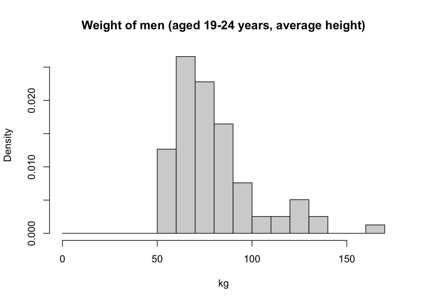
If we want to compare these data to a normal model, which particular normal
model should we choose?
That is, which mean and which standard deviation should we assume?
For the random numbers in our earlier example, we set a target mean and target
standard deviation with the arguments mean and sd inside rnorm().
As we saw last time, the mean and standard deviation of a sufficiently large
sample of random numbers hardly differs from the parameters specified in
rnorm(), so it’s natural to set the mean and standard deviation in the
curve() function equal to the arguments passed to rnorm().
When we work with real data, we neither know the mean nor the standard
deviation of the random process that generated the data, so we must first
compute the mean and standard deviation from the sample before we can draw a
bell curve.
Let me follow the textbook’s notation.
I call the mean of the data y_bar and the standard deviation s.
y_bar <- mean(weight)
s <- sd(weight)
Next we add the bell curve of a normal model with mean y_bar and standard
deviation s.
hist(weight,
     breaks = seq(0, 170, 10),
     freq = FALSE,
     main = "Weight of men (aged 19-24 years, average height)",
     xlab = "kg")
curve(dnorm(x, mean = y_bar, sd = s),
      from = 0,
      to = 170,
      add = TRUE,
      col = "red")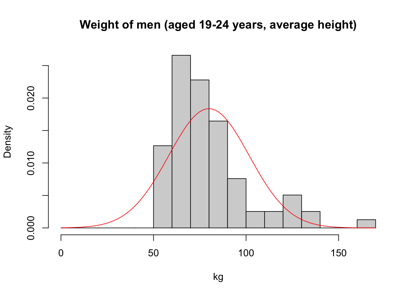
From this plot, we conclude that the data are too right-skewed to come from the normal model. Some histogram bins on the right are higher than predicted by the model, and the peak of the data is too far to the left.
Plotting a bell curve on top of a histogram is a great diagnostic tool for
detecting deviations from a normal model.
Another tool to visually assess whether a normal model fits empirical data is
the so-called “normal probability plot”, also known as quantile-quantile plot
or Q-Q plot.
In R, we create a normal probability plot with qqnorm().
Here is, for example, the normal probability plot for our set of normally
distributed random numbers.
qqnorm(r)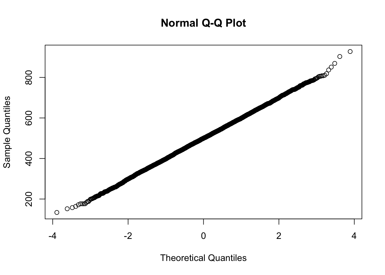
A normal probability plot represents every data point in the sample by one point on the plot. On the vertical axis, the plot shows the quantile of a data point in the observed distribution of values. Along the horizontal axis, the plot shows the “theoretical quantile” (i.e. the quantile if the data were strictly normally distributed with the same mean and the same standard deviation). If the data are approximately normal, the points in the normal probability plot are located close to a straight line.
Unsurprisingly, the points in this plot are almost exactly on a straight line
because the sample was generated from a normal model.
We can add the line to the plot with qqline().
Let’s change the line colour from the default, which is black, to red so that
we can see the line more clearly on a background of black points.
qqnorm(r)
qqline(r, col = "red")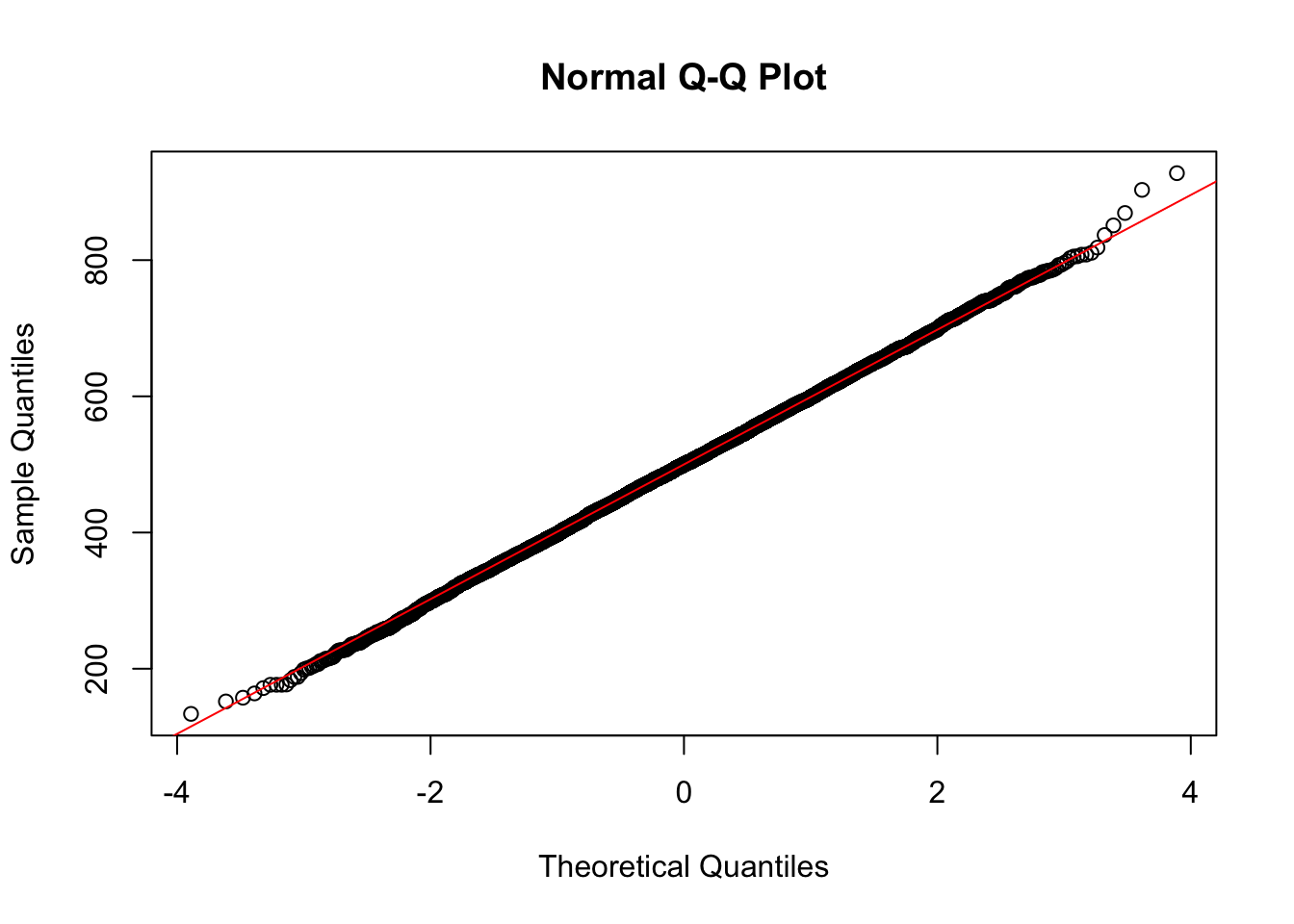
Real-world data, by contrast, are hardly ever on a perfect line. Here is the Q-Q plot for the body weight data.
qqnorm(weight)
qqline(weight, col = "red")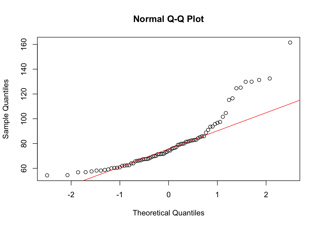
If the data look as clearly curved as in this normal probability plot, we should look at a histogram of the data to diagnose in which way the data differ from a normal model. As we saw from the histogram, the problem in this example is that the distribution is too right-skewed.
In summary, we learned two visualisation strategies to assess whether a normal model fits quantitative data.
- We can make a histogram with
hist()and the argumentfreq = FALSE. Then we add the bell curve of a normal model with thecurve()function. Inside thecurve()function, we must use the argumentadd = TRUEso that the bell curve appears in the same plot as the histogram. - Alternatively, we can make a normal probability plot with
qqnorm(). If the data are consistent with a normal model, the data points are close to the line that we obtain with theqqline()function. Otherwise we should look at a histogram to determine in which way the distribution of the data deviates from a normal model.
In our next tutorial, we learn how we calculate the correlation between two quantitative variables.
See you soon.