Chapter 28 Calculating Correlation Coefficients with R

Welcome back to Quantitative Reasoning! When we collect data, we often have more than one quantitative variable for each observation. An important question is whether these quantitative variables are associated with each other. For example, we may want to find out whether there’s a statistical association between body height and hip circumference. Or we may want to know whether brighter stars tend to have higher masses, or whether higher salaries are associated with more donations to charities. Our textbook introduces an important measure for the linear association between two quantitative variables: the correlation coefficient.

In this tutorial, we’ll learn how to visually assess with a scatter plot matrix which quantitative variables in a data frame are linearly associated with each other. We’ll learn how to calculate the correlation coefficient with the R function cor(). We’ll see examples of using cor() for a single pair of variables and for all pairs of variables in a data frame. We’ll also learn different options for excluding missing values from the calculation.

As a concrete example, we work with a data set extracted from the 2017-2018 US National Health and Nutrition Examination Survey (NHANES). There were 230 female participants aged between 20 and 25 years. For each participant, data were collected about body measures to estimate the prevalence of overweight and obesity. You can find the spreadsheet at the URL below this video (http://michaelgastner.com/data_for_QR/body_measurements.csv). Let’s import the data and shorten the name of the data frame to bm.

bm <- read.csv("body_measurements.csv")

This data frame has four columns: body height, upper arm length, arm circumference and hip circumference. All measurements are in centimetres.

head(bm)

##   height upper_arm_length arm_circum hip_circum
## 1  158.4             36.0       26.5      101.1
## 2  164.7             38.1       30.5       97.4
## 3  156.9             34.0       28.5      101.7
## 4  158.1             35.0       22.2       88.7
## 5  158.2             35.0       32.0      100.3
## 6  162.0             34.4       32.7       99.3

Before we calculate the correlation coefficient for a pair of variables, we should always check whether the association between the variables is approximately linear. The easiest way to make this check is to look at a scatter plot. Let’s apply our knowledge from tutorial 22 to make a scatter plot of upper arm length versus height.

plot(upper_arm_length ~ height,
     data = bm,
     main = "Upper Arm Length vs. Body Height of Women (Age 20-25)",
     xlab = "Body height (cm)",
     ylab = "Upper arm length (cm)")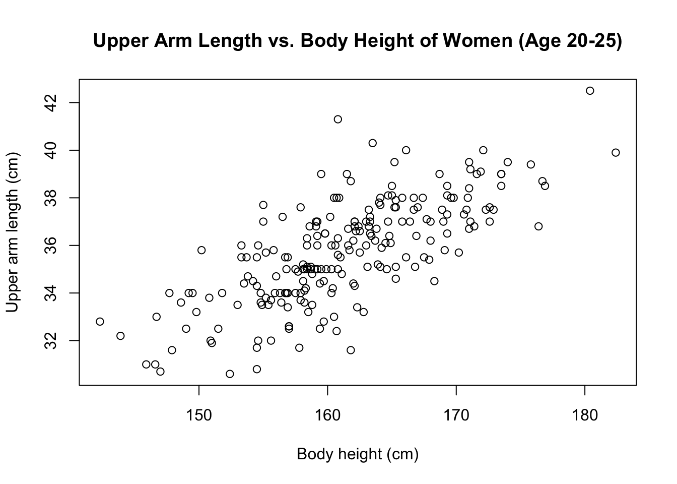

This scatter plot reveals that upper arm length tends to increase as a function of body height. There’s substantial spread in these data but no discernible curvature, so it’s appropriate to summarise the association in terms of the correlation coefficient. R calculates the correlation coefficient with the function cor(). In its basic form, cor() needs two inputs: the x-coordinates and the y-coordinates.

cor(bm$height, bm$upper_arm_length)

## [1] NA

The result of cor(bm$height, bm$upper_arm_length) is NA because at least one of the two input vectors contains missing values. For example, the upper arm length in row 52 is NA. In tutorial 18, we learned how to exclude missing values from the calculation of summary statistics (e.g. mean or standard deviation): we added the argument na.rm = TRUE. As I explain later in this tutorial, the situation is a little bit more complicated when we want to exclude missing values from the calculation of the correlation coefficient. It turns out that, instead of na.rm = TRUE, we should pass the argument use = "complete.obs" to cor(). The command cor(bm$height, bm$upper_arm_length, use = "complete.obs") returns the correlation coefficient for all survey participants for whom we know both body height and upper arm length.

cor(bm$height, bm$upper_arm_length, use = "complete.obs")

## [1] 0.7300344

The positive return value indicates that upper arm length tends to increase as a function of height. Remember that a correlation coefficient of 1 implies that all data points fall exactly on a straight line with positive slope. In our case, there is some scatter in the data, so the correlation coefficient must be less than 1. Still, the observed correlation is moderately strong.

Suppose we want to know the correlation coefficients for all pairs of columns in the data frame bm. We could make a scatter plot for each pair. If the association between the two variables is roughly linear, we can calculate the corresponding correlation coefficient with cor() for this specific pair of variables. However, going through each pair separately is time-consuming. If a data frame contains only numeric columns, we can generate scatter plots for all pairs of columns by passing the data frame as first argument to the plot() function. For example, plot(bm, ...) produces twelve different scatter plots with a single command. We may wish to expand the Plots tab to see the data in detail.

plot(bm, main = "Body Measures in 2017-2018 NHANES")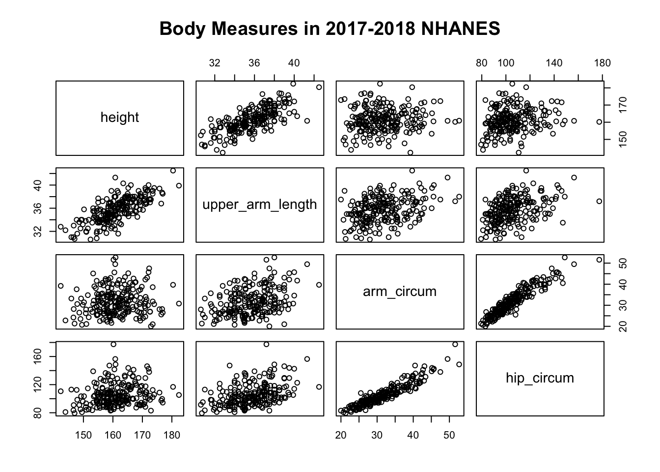

The plots are arranged in a tabular format known as a scatter plot matrix. For example, the plot in the first row and third column shows a scatter plot of the variable in the first column of bm (i.e. height) as a function of the variable in the third column (i.e. arm circumference).

Scatter plot matrices are great tools for exploratory data analysis. We can quickly determine which pairs of variables are roughly linearly associated. We can also visually assess the spread in the data. For example, arm circumference and hip circumference appear to be more strongly correlated than height and arm circumference. None of the plots in the scatter plot matrix reveals an outlier or clear curvature in the data. Consequently, the correlation coefficient is a meaningful quantity for each pair of variables in this example.

As we’ve just seen, we can pass a purely numeric data frame as input to the plot() function. The same is true for the cor() function. Instead of calculating the correlation coefficient for each pair of columns with a separate call of cor(), we receive all correlation coefficients with a single command if we pass the data frame as first argument.

cor(bm)

##                  height upper_arm_length arm_circum hip_circum
## height                1               NA         NA         NA
## upper_arm_length     NA                1         NA         NA
## arm_circum           NA               NA          1         NA
## hip_circum           NA               NA         NA          1

The result of cor(bm) is a tabular arrangement of the correlation coefficients. For example, the number in the first row and third column shows the correlation coefficient of height and arm circumference.

At this stage, the correlation matrix looks a little bit disappointing. All correlation coefficients are NA except the correlation coefficient of a variable with itself, which is of course equal to 1. The NAs are the results of missing values in bm. As we learn now, we can remove missing values in different ways, depending on whether we want to completely exclude a row with an NA or whether we want to exclude only those pairs of numbers that actually contain NA. Let’s take a look at two examples.

In row 52 of bm, the only known measure is height. The remaining three variables are missing.

bm[52, ]

##    height upper_arm_length arm_circum hip_circum
## 52  163.5               NA         NA         NA

Consequently, any possible pair of variables that we can form from these four values contains NA. If we decide to remove missing values before calculating the correlation coefficient, this entire row should be removed because it contains no useful information.

The situation is more complicated in row 32, where hip circumference is the only missing variable.

bm[32, ]

##    height upper_arm_length arm_circum hip_circum
## 32  173.5               39         21         NA

When we calculate the correlation coefficient of hip circumference and any other variable, we should exclude this row if we don’t want the result to be NA. Still, we can form pairs of variables that don’t involve an NA from this row (e.g. height and upper arm length). In some applications, we may want to include partial information from this row. In other cases, it may be more appropriate to exclude this row entirely.

Because there are different strategies for removing missing values, it wouldn’t be sensible for the cor() function to have an argument na.rm that can only be TRUE or FALSE. Instead, cor() has a different argument, called use, which can accept a variety of arguments. The two most important arguments for us are "complete.obs" and "pairwise.complete.obs". If we set use = "complete.obs", row 32 is entirely removed from the calculation. If we set use = "pairwise.complete.obs", row 32 is only ignored for pairs of variables that involve NA (i.e. any combination of hip circumference with another variable).

When we compare the results of these two options in the cor() function, we receive slightly different answers.

cor(bm, use = "complete.obs")

##                     height upper_arm_length arm_circum hip_circum
## height           1.0000000        0.7259228  0.1061935  0.1942494
## upper_arm_length 0.7259228        1.0000000  0.3843140  0.4187889
## arm_circum       0.1061935        0.3843140  1.0000000  0.9332575
## hip_circum       0.1942494        0.4187889  0.9332575  1.0000000

cor(bm, use = "pairwise.complete.obs")

##                      height upper_arm_length arm_circum hip_circum
## height           1.00000000        0.7300344 0.09158687  0.1942494
## upper_arm_length 0.73003442        1.0000000 0.36746497  0.4187889
## arm_circum       0.09158687        0.3674650 1.00000000  0.9332575
## hip_circum       0.19424938        0.4187889 0.93325754  1.0000000

There’s no simple rule whether it’s more appropriate to choose "complete.obs" or "pairwise.complete.obs". For the data sets that we encounter in this course, the differences are generally small. In both cases, we conclude that arm circumference and hip circumference are more strongly correlated than height and arm circumference. This result is consistent with our earlier judgment based on the scatter plot matrix.

If we apply cor() to two vectors instead of a data frame, it doesn’t matter whether we remove missing values with use = "complete.obs" or use = "pairwise.complete.obs". In that case, every complete observation is also a pairwise complete observation and vice versa. For example, if we insert bm$height as first argument into cor() and bm$upper_arm_length as second argument, the result must be the same regardless of whether we choose use = "complete.obs" or use = "pairwise.complete.obs".

cor(bm$height, bm$upper_arm_length, use = "complete.obs")

## [1] 0.7300344

cor(bm$height, bm$upper_arm_length, use = "pairwise.complete.obs")

## [1] 0.7300344

I prefer the option with "complete.obs" because it needs less typing, but both options lead to the same outcome.

Here is a summary of this tutorial.

We learned that the plot() function can accept a data frame as first argument. If the data frame only contains numeric columns, the result is a scatter plot matrix. If a data frame has non-numeric columns, we should remove them before passing the data frame as argument to the plot() function. Otherwise the plot isn’t easily interpretable.
We learned that we can calculate the correlation coefficient of two equally long numeric vectors x and y with cor(x, y). If x or y contain missing values, we can remove them from the calculation with the additional argument use = "complete.obs".
If we have a purely numeric data frame dfr, we can calculate the correlation coefficients for all pairs of variables with cor(dfr). We can remove missing values with the argument use. If we want to remove all rows with at least one missing value from the calculation, we set use = "complete.obs". If we want to include all pairs of non-missing values in the calculation, we set use = "pairwise.complete.obs".

In this tutorial, we learned how we can calculate the correlation coefficient, which is a measure for the tendency of two variables to exhibit an increasing or decreasing linear trend. In our next tutorial, we learn how we can fit a line that describes this trend.

See you soon.