Chapter 30 Extracting Information about a Linear Model
Welcome back to Quantitative Reasoning! In the previous tutorial, we learned how to build a linear model, extract its coefficients and plot the regression line on a scatter plot. In this tutorial, we’ll learn how to obtain further numeric information about the model. We’ll also learn how to make a residual plot.
Last time, we fitted a linear model for upper arm length as a function of body height. You can click on the link below this video to access the data again (http://michaelgastner.com/data_for_QR/body_measurements.csv). Here are the commands we used last time.
bm <- read.csv("body_measurements.csv")  # Import data
model <- lm(upper_arm_length ~ height, data = bm)  # Fit linear model
plot(upper_arm_length ~ height,
     data = bm,
     main = "Upper Arm Length vs. Body Height of Women (Age 20-25)",
     xlab = "Body height (cm)",
     ylab = "Upper arm length (cm)")
abline(model, col = "red")  # Add regression line
I mentioned in our previous tutorial that the function lm() returns a data
structure of class lm, which is more complicated than a vector or a data
frame.
When we type the variable name model in the console and press the return
key, R only reveals the y-intercept and the slope, which are only the tip of
the iceberg.
model##
## Call:
## lm(formula = upper_arm_length ~ height, data = bm)
##
## Coefficients:
## (Intercept) height
## -1.1579 0.2289R prints out more information when we run summary(model).
summary(model)##
## Call:
## lm(formula = upper_arm_length ~ height, data = bm)
##
## Residuals:
## Min 1Q Median 3Q Max
## -4.2701 -0.9272 -0.0276 0.9211 5.6587
##
## Coefficients:
## Estimate Std. Error t value Pr(>|t|)
## (Intercept) -1.15788 2.34294 -0.494 0.622
## height 0.22885 0.01451 15.772 <2e-16 ***
## ---
## Signif. codes: 0 '***' 0.001 '**' 0.01 '*' 0.05 '.' 0.1 ' ' 1
##
## Residual standard error: 1.499 on 218 degrees of freedom
## (10 observations deleted due to missingness)
## Multiple R-squared: 0.533, Adjusted R-squared: 0.5308
## F-statistic: 248.8 on 1 and 218 DF, p-value: < 2.2e-16During this course, we can only scratch the surface of the statistical
information contained in R’s output.
An easily interpretable piece of information is “Multiple R-squared”, which
our textbook simply refers to as \(R^2\) in chapter 7.6.
It can be interpreted as the fraction of the data’s variance that is accounted
for by the linear model.
If we want to see only the \(R^2\)-value and omit the remaining output from
the summary() function, we use the command summary(model)$r.squared.
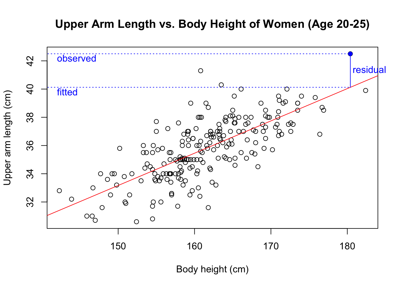
summary(model)$r.squared## [1] 0.5329503We conclude that 53.3% of the data’s variance is explained by the linear model. The remaining 46.7% are due to the scatter of the residuals. As our textbook explains in chapter 7.1, the residual of an observation is the observed value minus the predicted value. This plot shows the residual of the data point highlighted in blue.
We can obtain the residuals for all observations with the function
residuals().
residuals(model)The residuals play a key role in assessing whether a linear model is a good
description of our data.
Our textbook suggests that we should always make a scatter plot of the
residuals after fitting a linear model.
In figure 7.5 on page 209, our textbook uses the observed values for the
predictor variable as x-coordinates, whereas the unnumbered figure on page 215
has the predicted outcomes on the x-axis.
The only difference between using the observed predictor or predicted outcome
is a linear scaling of the x-axis, which doesn’t affect the conclusions we
draw from the plot.
Using the predicted values as x-coordinates is generally more common in the
literature.
It’s also easier to produce such a plot with R, especially if the data contain
missing values, as it’s the case in our example.
We can simply use the plot() function with the linear model as first
argument and which = 1 as second argument.
Don’t worry too much about the meaning behind which = 1.
There are various diagnostic plots that the plot() function can produce for
a linear model.
With the arguments which = 2, which = 3 etc., we get other types of
diagnostic plots.
In this course, we only need the residual plot, so we’ll generally work with
the argument which = 1.
plot(model, which = 1)
As usual, we can add a main title to the plot with the argument main.
We can also change the cryptic formula on the second line of the x-axis
label with the sub.caption argument.
plot(model,
     which = 1,
     main = "Upper Arm Length Predicted from Body Height",
     sub.caption = "Upper arm length (cm)")
If the linear model is appropriate for a data set, then the point pattern in the residual plot shouldn’t have any noticeable curvature. As a visual aid to judge whether the data are curved, R inserted a red LOWESS curve into the plot. In our example, the LOWESS curve is nearly straight, which indicates that the data satisfy the “straight-enough condition” of our textbook.
Another condition for applying a linear model is that there are no outliers
that would affect the linear trend.
R writes the indices of the three most extreme outliers next to the
corresponding points in the plot.
For example, the upper arm length of the participant in row 198 of bm has a
large positive residual.
It’s always a good idea to check whether there’s something interesting or
suspicious about outliers.
In this example, data point 198 doesn’t have much influence on the line that
we fit to the data, so there’s no compelling reason to take any special action
regarding this data point.
Another condition on the residual plot is that the plot doesn’t thicken. That is, the spread in the y-direction shouldn’t depend strongly on the x-value. The cloud of points should be equally thick on the left and on the right. If this condition is violated, we may need to re-express the data before fitting a linear model.
Our example satisfies all conditions for linear regression.
Consequently, it’s appropriate to use a linear model for upper arm length
as a function of body height.
Suppose that we encounter a group of 20-25 year-old women who aren’t in our
data set.
If we know their body heights, what would be our predictions for their upper
arm lengths?
In our next tutorial, we learn how to predict the y-coordinate for a given
x-coordinate with the function predict().
Let’s recap the main points of this tutorial.
- If a linear model is stored in the variable
model, thensummary(model)returns various statistical pieces of information. - We obtain the \(R^2\)-value with
summary(model)$r.squared. - We get a vector of the residuals with
residuals(model). - We make a residual plot with
plot(model, which = 1). A residual plot should satisfy the three conditions stated in chapter 7.7 of our textbook:- the “straight-enough” condition,
- the outlier condition and
- the “does-the-plot-thicken?” condition.
Next time we learn how we can make predictions on the basis of a linear model.
See you soon.