Chapter 31 Making Predictions on the Basis of a Linear Model
Welcome back to Quantitative Reasoning! During our previous three tutorials, we worked with a subset of the 2017-2018 NHANES data set for body measurements. There’s one set of measurements for each woman aged between 20 and 25 years who participated in the survey. You can find the data at the URL below this video (http://michaelgastner.com/data_for_QR/body_measurements.csv). Last time, we looked at the residual plot for the linear model of upper arm length as a function of body height. Here are the commands to reproduce the residual plot.
bm <- read.csv("body_measurements.csv")
model <- lm(upper_arm_length ~ height, data = bm)
plot(model,
     which = 1,
     main = "Upper Arm Length Predicted from Body Height",
     sub.caption = "Upper arm length (cm)")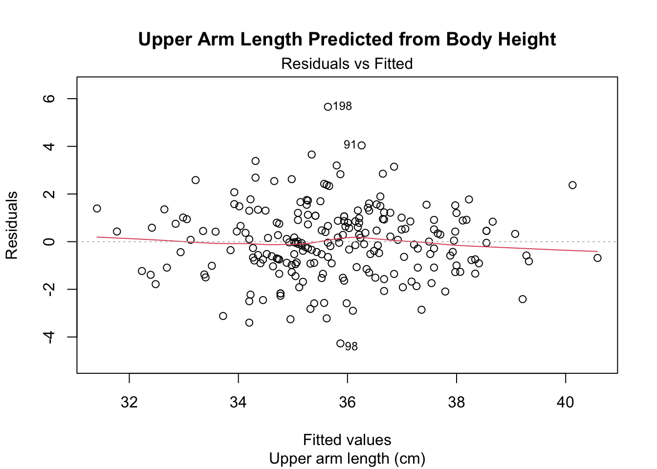
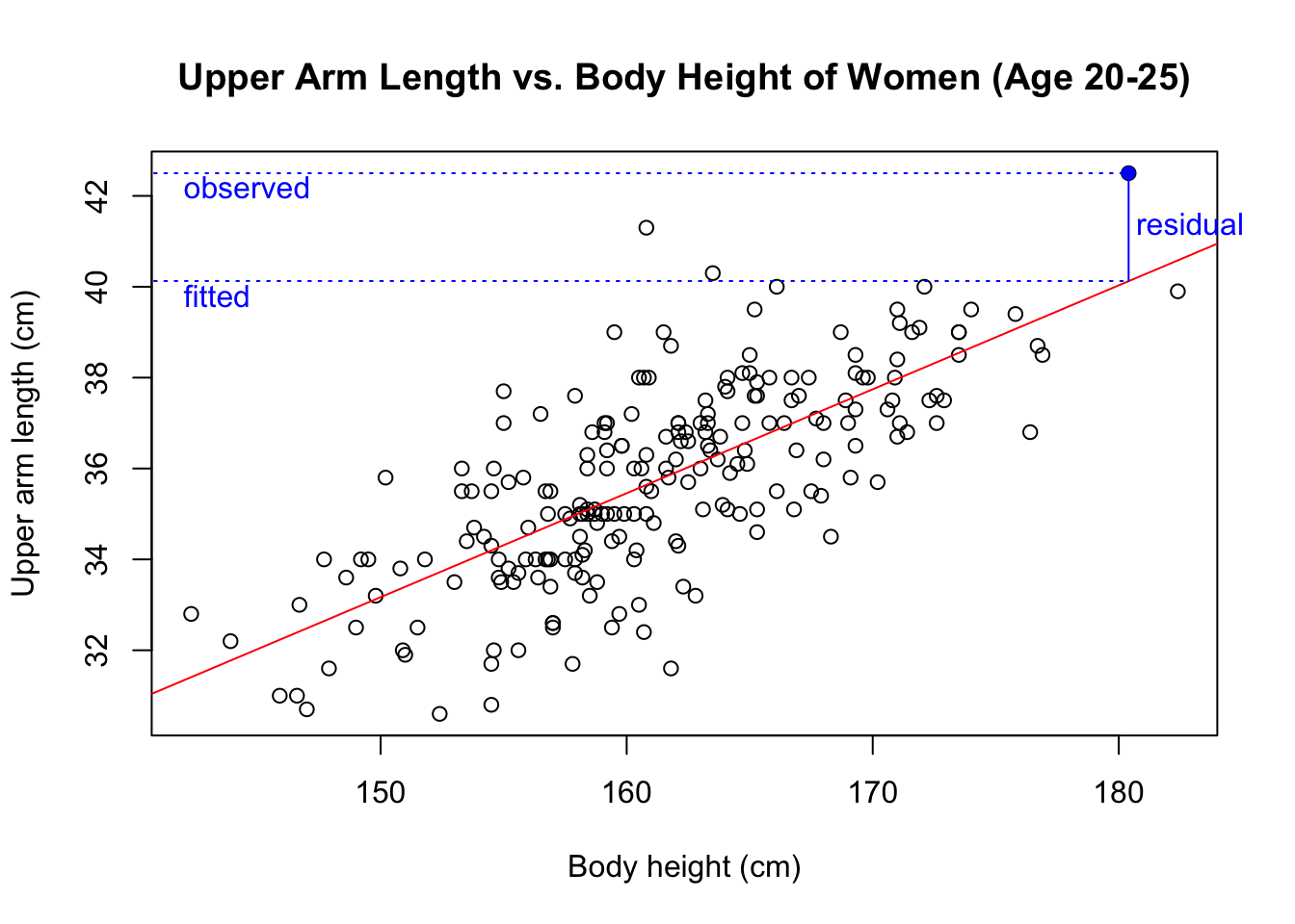
The x-coordinates are fitted values (i.e. the upper arm length that is predicted on the basis of a participant’s body height). In the scatter plot of the observed upper arm length versus the body height, the fitted upper arm length is the y-value of the regression line for a given body height. For example, this plot shows the fitted upper arm length of the blue data point.
For the purpose of making the residual plot, R automatically calculated the
fitted values for us, but sometimes we would like to determine predicted
values ourselves.
In principle, we can determine the predicted values from the y-intercept and
the slope of the regression line, but R offers a more convenient way for this
task: the function predict().
The first argument in predict() is the fitted linear model, usually
calculated with the function lm().
In our script, we gave the fitted linear model the variable name “model”.
If model is the only argument passed to predict(), the return value is a
vector that contains the fitted y-values for the observed x-values in the
data set, which is in our case the data frame bm.
predict(model)For example, the linear model predicts an upper arm length of 35.09 cm
for the participant in row 1 of bm.
head(predict(model))## 1 2 3 4 5 6
## 35.09204 36.53380 34.74877 35.02339 35.04627 35.91590This prediction is based on her body height, which is 158.4 cm.
bm[1, ]## height upper_arm_length arm_circum hip_circum
## 1 158.4 36 26.5 101.1Her true upper arm length is 36 cm, close to the predicted value of 35.09 cm.
Calculating the fitted y-values of the participants in the study can be useful, but it’s even more interesting to predict upper arm lengths for women who weren’t part of the sample. Suppose we know the body height of a woman in the same age group as the study participants, but we don’t know her upper arm length. What is our prediction?
Suppose we want to make predictions for three women with body heights of
155.2 cm, 158.9 cm and 165.1 cm.
Let’s fill these values into an object called measurements.
The predict() function expects these predictions to be in a column of a data
frame.
The column name must match the name of the variable that we used as a
predictor when we built the linear model with lm().
In our example, we used the formula upper_arm_length ~ height, so the column
in the data frame must be called height.
# Objective: predict upper arm lengths for heights 155.2, 158.9, 165.1
measurements <- data.frame(height = c(155.2, 158.9, 165.1))
We can pass measurements as a second argument to predict().
The name of this argument is newdata.
predict(model, newdata = measurements)## 1 2 3
## 34.35972 35.20647 36.62534The result shows that the linear model predicts an upper arm length of
34.36 cm for the first woman in the data frame measurements, 35.21 cm for
the second woman and 36.63 cm for the third.
Of course, we would have obtained the same values if we had inserted the
body heights into the equation for the regression line:
\(-1.1579 + 0.2289\cdot\text{height}\).
coef(model)## (Intercept) height
## -1.1578759 0.2288505However, using the predict() function makes the intention of our calculation
more obvious to somebody else who reads our R script.
It may feel awkward that we must put the three measurements into a data frame.
Why doesn’t R allow us to pass a simple vector as newdata argument?
The answer is that the function predict() is designed to handle general
statistical models that may rely on multiple predictor variables.
For example, we may want to build a model that predicts upper arm length on
the basis of arm circumference as well as body height.
For a model with multiple predictor variables, it makes sense to enter
different variables as different columns of a data frame.
For our model, which only has body height as a single predictor, this approach
may feel indirect, but in the end we get the information we’re looking for.
In summary, we use the predict() function to obtain predictions on the basis
of a linear model.
The first argument of predict() is a concrete linear model, usually
calculated with lm() before we run predict().
If the linear model is the only argument passed to predict(), R returns
the fitted values for the observations that we passed as arguments to lm().
If we want to get predictions for a new set of observations, we must create
a data frame in which R can find the predictor variable as a column name.
Then we pass this data frame as a second argument, called newdata, to the
predict() function.
Predictions are, of course, generally different from the truth. In reality, we usually encounter a certain degree of randomness. Next time we learn how we can use R to generate random samples from a finite set of objects.
See you soon.