Chapter 29 Fitting a Linear Model
Welcome back to Quantitative Reasoning! In our previous tutorial, we learned how to visually assess whether two quantitative variables are linearly associated. If there’s no curvature in the scatter plot and there are no outliers that substantially influence the linear trend, then the correlation coefficient is a meaningful summary of the association between the two variables. Last time, we learned how to calculate the correlation coefficient with R, but we haven’t yet learned how we can fit a line to the data. This topic is the central learning outcome of this tutorial.
Last time, we made this scatter plot of upper arm length as a function of body height. You can retrieve the data from the URL below this video (http://michaelgastner.com/data_for_QR/body_measurements.csv).
bm <- read.csv("body_measurements.csv")
plot(upper_arm_length ~ height,
     data = bm,
     main = "Upper Arm Length vs. Body Height of Women (Age 20-25)",
     xlab = "Body height (cm)",
     ylab = "Upper arm length (cm)")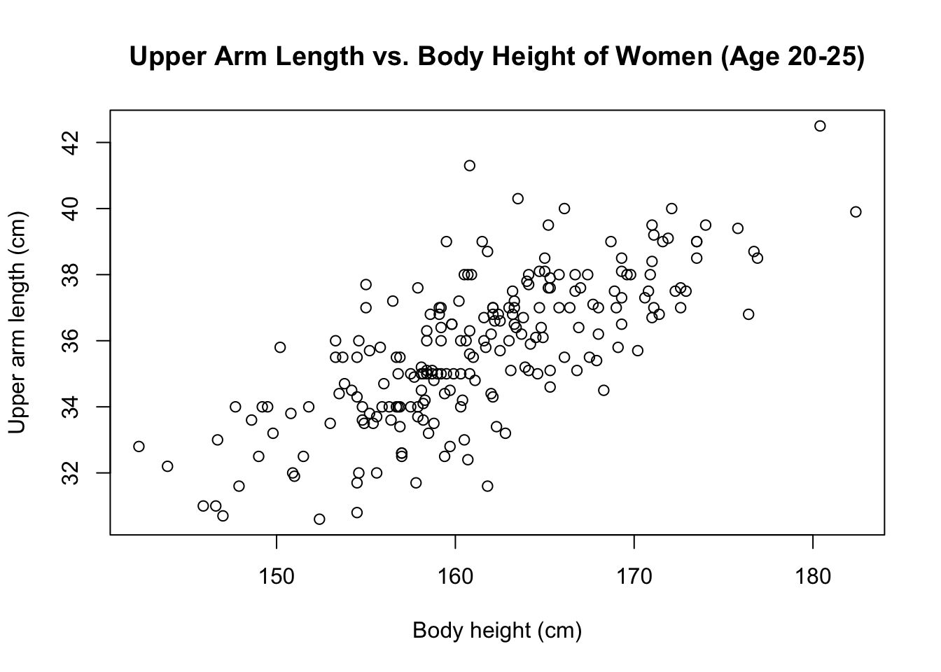
These data are suitable for a linear model because there’s no noticeable
curvature, and there are no extreme outliers whose presence would strongly
influence the linear trend.
Let’s go ahead and fit a line to these data.
Conventionally, the line of best fit is defined as the line that minimises the
sum of the squared residuals.
For historical reasons, this line is also called a least-squares regression
line.
You can find more background information about linear regression in chapter 7
of our textbook.
In R, we fit a linear model with the function lm().
The first argument of lm() is a formula containing a tilde.
For example, here is how we model upper arm length as a function of body
height.
lm(bm$upper_arm_length ~ bm$height)The order of the variables in lm() is important.
The variable to the left of the tilde (i.e. upper arm length) is the quantity
we’re trying to predict on the basis of the variable to the right (i.e.
height).
If we interchange the variables, we build a different model that leads to
different conclusions.
There’s more information about the difference between the two models in
chapter 7.6 of our textbook.
In our example, both vectors in the formula are from the data frame bm.
If we don’t want to repeat the name of the data frame in the formula, we can
enter the name as an optional data argument.
lm(upper_arm_length ~ height, data = bm)##
## Call:
## lm(formula = upper_arm_length ~ height, data = bm)
##
## Coefficients:
## (Intercept) height
## -1.1579 0.2289The output shows that the least-squares regression line has the equation
\[
\text{upper arm length} = -1.1579 + 0.2289 \cdot \text{height}.
\]
The first number (i.e. \(-1.1579\)) is called the y-intercept, and the second
number (i.e. \(0.2289\)) is called the slope of the regression line.
We can save the result of lm() as a variable (e.g. called model).
model <- lm(upper_arm_length ~ height, data = bm)The data structure of model is more complicated than the vectors and data
frames we’ve seen so far.
In technical terms, model is an object of class lm.
Details about this special data structure are beyond the scope of this course.
It will be sufficient to learn a few functions that accept such objects as
input and return useful output.
One such function is coef().
It returns the two coefficients of the regression line (i.e. y-intercept and
slope).
coef(model)## (Intercept) height
## -1.1578759 0.2288505We can use square brackets for subsetting.
For example, coef(model)[2] returns the slope.
coef(model)[2]## height
## 0.2288505Arguably, the most important action we want to perform after calculating a
linear model is to add the regression line to a scatter plot of the data.
We can accomplish this task by first running the plot() function as before,
and then we run the command abline(model).
The default colour of the line is black, which is difficult to see on a
background of black points, so let’s change the line colour (e.g. to red).
plot(upper_arm_length ~ height,
     data = bm,
     main = "Upper Arm Length vs. Body Height of Women (Age 20-25)",
     xlab = "Body height (cm)",
     ylab = "Upper arm length (cm)")
abline(model, col = "red")
The line in the plot confirms that an increase in body height tends to be associated with an increase in upper arm length.
Here is a summary of this tutorial.
- We learned that we fit a linear model of
yas a function ofxwithlm(y ~ x). The order of the variables is important. Predictingyas a function ofxis fundamentally different from predictingxas a function ofy. - If the data are from two columns of the same data frame
dfr, we can use an optionaldataargument. For example, if we want to model the columndfr$was a function ofdfr$v, we can build a linear model withlm(w ~ v, data = dfr). - We can extract the coefficients of the regression line with
coef(). - We can add the regression line to a scatter plot with
abline().
There are many other functions with which we can extract information about a linear model. We cover some of them in the next tutorial.
See you soon.